Predicting Home Prices

Our K-means analysis shows that, on average, otherwise similar homes are worth about 18% more in highway towns than in non-highway towns.

But what does this mean for my in-laws, specifically? To answer this, I predicted their new home value using a random forest regression.

My model was trained and tested on 76,000 home sales in highway towns, based on the following features:

• acreage
• livable square footage
• year of sale
• year built
• story height
• style of the home
• distance to NC-540
• distance to the Raleigh city center
• and distance to the RDU airport

Home attributes, such as acreage, liveable square footage, style, story height, and year of build and sale are all typical features to include in a hedonic model of a home’s value. I included the distance to NC-540 because of its importance to our central research question.

I included the distance to the Raleigh city center as a way for the model to differentiate between homes that are a similar distance from NC-540, but may be within (closer to the city center) or outside the beltway (further from the city center). This spatial difference is likely to have a different home value outcome.

Finally, I included the distance to the RDU airport as a way to try and account for the spatial fixed effects of the highway towns. Since I couldn’t include the towns themselves in my model (because then it would be impossible to predict for my in-laws’ home, which isn’t in one of these towns), I used distance from the airport as a continuous variable to approximate this effect instead. The highway towns are all closer to the RDU airport than the non-highway towns; perhaps there is something about proximity to the airport or another nearby spatial feature that explains the higher home values in this area.

Error Metrics

After cross-validation, my model had a mean R-squared of 0.885, meaning that my model accounts for 88.5% of the variation in home prices within highway towns. My model had a mean absolute error (MAE) of $28,704, meaning that on average, its prediction was off by almost $29,000. Its accuracy was 84%, meaning that it accurately predicts highway towns’ home prices 84% of the time.

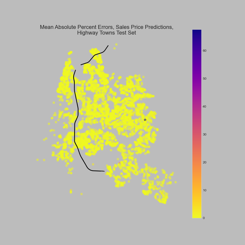
The map below shows the mean absolute percent error (MAPE) for each home, for a random sample of 5000 homes in the test set. The majority of predictions see less than 10% MAPE, while a few outliers see much higher errors.

For a relatively simple set of features, I thought these metrics were unusually high; so I ran a simple linear regression to confirm if these features really did as good of a job predicting home prices. They did: my linear model had an R-squared of 81%, indicating that the more complex random forest regression model’s score of 88.5% is reasonable.

Which features were most important?

The table below shows the importances of my included features to the model’s prediction of sale prices. Note, home styles has been removed from this list since its importance was smaller than 0.001.

Liveable square footage was by far the strongest predictor of a home’s value. This feature explained 64.4% of the variance in house prices for homes in highway towns. At first, I thought this might be because of higher housing density: if homes are smaller, then square footage would be more valuable. However, the average home size in these towns is almost 2500 sqft – quite large. It seems that square footage is so valuable in these towns because there is something about these towns that people want.

In second place came the sale year, at 19%. Since real estate saw a boom in sales in 2020 and 2021, this is not surprising. Distance to the highway was only the fifth most important feature, at 2.1%. Therefore, a home’s value is based more on the general trend of real estate in the area than on the distance to the highway.